Posted in Engineering

Best Database-as-a-Service Platforms for Developers in 2026: PlanetScale vs Neon vs Supabase

Every one of the major serverless database platforms has rewritten its pricing and features at least once in the past two years, which makes “just use whichever one a tutorial mentions” a riskier strategy than it used to be. PlanetScale killed its free tier, Neon was acquired by Databricks for roughly $1 billion, and Supabase pushed its Team plan to $599 a month while keeping a genuinely usable free tier underneath it. Here is where the three stand as of late 2026, based on each vendor’s current pricing pages.

At a Glance

PlatformDatabase engineFree tierEntry paid priceBranching model
PlanetScaleMySQL (Vitess) or Postgres (single-node, HA, or sharded Neki)None — discontinued March 2024Postgres single-node from $5/month; Metal from $50/monthFull schema + data branching with non-blocking “deploy requests” across all three products
NeonPostgres onlyYes — 100 projects, 100 CU-hours/project/monthPay-as-you-go from $0.106/CU-hour (Launch)Copy-on-write branches; child branches start at $0 storage
SupabasePostgres only, plus bundled Auth/Storage/Edge Functions/RealtimeYes — 2 active projects, 500 MB DB eachPro from $25/monthMigration-based branch cloning (schema, not data, by default)

Short Verdict

If you need MySQL at serious scale, or you specifically want PlanetScale’s online, reversible schema-change workflow, PlanetScale is still the strongest option — but you’ll pay from day one. If you want a free-to-start, true serverless Postgres with instant, storage-efficient branching, Neon is the cleanest fit, and it now sits inside Databricks’ data platform. If you want a database plus auth, storage, and realtime in one SDK and don’t mind a steep jump from $25 to $599 a month once you need SOC 2 compliance, Supabase is the practical default for full-stack app teams.

What Each Platform Actually Is

PlanetScale was built by the team that created Vitess, the MySQL-sharding layer YouTube uses internally, and that heritage still shapes the product. Its core pitch is non-blocking schema migrations: you branch a database, make schema changes on the branch, and merge them back through a reviewable “deploy request” that applies without locking tables or causing downtime. PlanetScale has since added single-node and high-availability Postgres, plus Neki, a newer sharded Postgres engine, so branching and online schema changes now work across both MySQL and Postgres. There is no serverless or usage-based free option; PlanetScale’s own support documentation confirms the free Hobby plan was discontinued in March 2024, and every new database lands on a paid plan immediately.

Neon is a Postgres-only platform built around separating compute from storage, which is what makes scale-to-zero and copy-on-write branching possible. In 2025, Databricks acquired Neon in a deal reported at roughly $1 billion, and Neon’s technology now also powers “Lakebase,” Databricks’ own managed Postgres product for agentic and transactional workloads inside the Databricks platform. Neon continues to operate its own pricing and product independent of that integration. Its free plan is genuinely free forever (no credit card required) and supports up to 100 projects, each with 100 compute-hours a month and autoscaling up to 2 compute units (about 8 GB RAM) before suspending after five minutes of inactivity.

Supabase bundles a full Postgres database with authentication, file storage, auto-generated REST and realtime APIs, and Edge Functions, positioning itself as “the Postgres development platform” and an explicit alternative for teams leaving Firebase. Every project is a real, portable Postgres instance underneath — row-level security and SQL are available from day one rather than hidden behind a proprietary query layer.

Branching, Compared Properly

“Branching” means three different things on these platforms, and the difference matters for cost and workflow:

  • PlanetScale branches are full copies used specifically for schema review: you make a DDL change on a branch, PlanetScale validates it, and a deploy request applies the change to production without locking tables, with a revert path if something goes wrong.
  • Neon branches are copy-on-write at the storage layer: creating a branch is near-instant and costs nothing until the branch starts diverging from its parent through new writes, because only the deltas are stored. Free and Launch plans include 10 branches per project; Scale allows more, and paid plans can scale to thousands of branches per project at $1.50 per extra branch-month.
  • Supabase branches clone configuration and schema (rebuilt from your migration history) but not data by default — you opt in to copying data with a seed file or an “Include data” setting. Preview branches tied to a pull request are deleted automatically on merge or close; persistent branches stick around for staging or QA.

For teams doing frequent, data-heavy branch testing, Neon’s copy-on-write model is the cheapest and fastest. For teams whose main pain point is risky schema migrations on a live MySQL database, PlanetScale’s deploy-request workflow is still the more mature, purpose-built tool — it’s worth comparing against dedicated database migration tools like Flyway, Liquibase, and Atlas if schema change safety is your main requirement rather than hosting itself.

Pricing and Free-Tier Reality

PlanetScaleNeonSupabase
Free tierNone100 CU-hrs/project/month, 1 GB storage/project, 20 GB/account, scale-to-zero after 5 min2 active projects, 500 MB DB each, pauses after 1 week inactive, 50k MAU auth
Cheapest paid tierPostgres single-node from $5/monthLaunch: pay-as-you-go, $0.106/compute-unit-hour, no monthly minimumPro: from $25/month, 8 GB included disk
Compliance-grade tierEnterprise, custom pricingScale plan adds private networking and higher capsTeam at $599/month adds SOC 2, ISO 27001, SSO, 14-day backups

Supabase’s jump from $25 to $599 a month purely to get SOC 2 and SSO is the single biggest line-item surprise in this comparison, and it’s worth budgeting for early if you’re selling into enterprise customers. Neon’s model is the most forgiving for prototyping, since usage is metered down to the compute-hour and idle projects cost nothing. PlanetScale’s lack of any free tier means it’s really a tool for teams who already know they need its specific migration workflow or Vitess-scale sharding, not a place to experiment for free.

Pros and Cons

PlanetScale

  • Pros: Best-in-class non-blocking schema migration workflow; proven MySQL sharding (Vitess) at extreme scale; now also offers Postgres and sharded Neki; strong uptime SLAs.
  • Cons: No free tier at all; pricing for Vitess/Neki/HA is custom and opaque; less beginner-friendly than Supabase or Neon for a first side project.

Neon

  • Pros: Genuinely free forever tier; fast, cheap copy-on-write branching; fine-grained compute-hour billing; backed by Databricks’ resources post-acquisition.
  • Cons: Postgres only, so no MySQL path; autoscaling ceiling on lower tiers can surprise teams that outgrow it quickly; being folded into Databricks’ roadmap (via Lakebase) adds some long-term direction uncertainty for standalone users.

Supabase

  • Pros: Database, auth, storage, realtime, and edge functions in one platform; real, portable Postgres with no proprietary lock-in; usable free tier; open source and self-hostable.
  • Cons: Free projects pause after a week of inactivity; branching doesn’t copy data by default; the $599/month Team plan is a steep cliff just to get compliance certifications.

Who It’s a Good Fit For

Choose PlanetScale if you’re running a high-traffic MySQL application and schema changes are a recurring source of downtime risk, or if you need proven horizontal sharding at YouTube-scale traffic. Choose Neon if you want Postgres with the cheapest possible branching for CI/preview environments and don’t want to pay for idle compute. Choose Supabase if you’re building a full-stack app and want auth, storage, and realtime bundled with your database rather than assembled from separate vendors.

Who Should Look Elsewhere

If you need a true free tier to experiment with zero commitment, skip PlanetScale entirely. If you need MySQL compatibility specifically, Neon and Supabase are both out, since both are Postgres-only. If your budget caps out well under $599/month but you still need SOC 2 for a sales deal, check Neon’s and PlanetScale’s enterprise terms directly, since compliance gating varies and changes often on all three platforms.

Bottom Line

There’s no single winner here — the three platforms have diverged rather than converged. PlanetScale is the specialist for safe, large-scale schema changes, especially on MySQL. Neon is the most cost-efficient, developer-friendly serverless Postgres, now with Databricks’ backing. Supabase is the most complete “backend in a box” for teams that want more than just a database. Match the pick to what’s actually slowing your team down today, not to whichever platform shows up first in a Twitter thread.

FAQ

Does PlanetScale have a free tier in 2026?
No. PlanetScale’s free Hobby plan was discontinued in March 2024, according to the company’s own support documentation. All databases now start on a paid plan immediately.

Is Neon still independent after the Databricks acquisition?
Neon operates as its own product with its own pricing, but Databricks acquired the company in 2025 for a reported $1 billion and has built “Lakebase,” a managed Postgres offering, on Neon’s underlying technology.

Can I use MySQL on Neon or Supabase?
No, both are Postgres-only. PlanetScale is the only one of the three with native MySQL (Vitess) support, alongside its newer Postgres offerings.

Does Supabase branching copy my production data?
Not by default. Supabase branches rebuild the schema from your migration history and start without data; you have to explicitly add a seed file or enable the “Include data” option to populate a branch.

Which platform is cheapest for a side project?
Neon, by a clear margin — its free tier has no card requirement and doesn’t pause projects for inactivity the way Supabase’s free tier does, and PlanetScale has no free tier at all.
Sources

Posted in Engineering

Vector Databases and Approximate Nearest Neighbor Search Explained: HNSW vs IVF for AI Retrieval

Every retrieval-augmented generation (RAG) pipeline, semantic search box, and recommendation engine built since 2023 depends on the same underlying problem: given a query vector, find the handful of vectors in a database of millions (or billions) that are closest to it. Doing this exactly, by comparing the query to every stored vector, is called k-nearest neighbor (kNN) search, and it does not scale — brute-force comparison is O(N) per query. So almost every real vector database instead does approximate nearest neighbor (ANN) search: trading a small, tunable amount of recall for orders-of-magnitude faster lookups. Two families of ANN algorithm dominate production systems in 2026: graph-based methods, led by HNSW, and partition-based methods, led by IVF. This piece explains how each actually works, what their real trade-offs are, and when to reach for which.

At a Glance

FactorHNSW (graph-based)IVF (partition-based)
Core ideaMulti-layer navigable graph; search by walking edges toward the queryCluster vectors into cells with k-means; search only the nearest cells
Key build parametersM (connections per node), efConstructionnlist (number of cells)
Key query parameterefSearchnprobe (cells searched)
Query speedVery fast, roughly logarithmic in dataset sizeFast, scales with nprobe/nlist fraction scanned
Memory overheadHigher — stores the full graph on top of vectors (~M × 2 × 4 extra bytes/vector)Lower — mainly list IDs plus chosen vector encoding
Build timeSlower to build, especially at high M/efConstructionFaster to build; k-means training step is comparatively cheap
Handles deletions well?No — removing nodes breaks the graph structureYes — easier to add/remove vectors from a cell
Typical usersQdrant, Weaviate, Milvus (default), pgvector (HNSW index)FAISS, Milvus (IVF variants), many large-scale offline pipelines

Why Exact Search Doesn’t Scale

An embedding model turns text, images, or audio into a dense vector, typically a few hundred to a few thousand floating-point numbers, positioned so that semantically similar inputs land close together under a distance metric like cosine similarity or Euclidean distance. Finding the true nearest neighbors to a query vector means computing that distance against every vector in the collection. At a few thousand vectors this is trivial. At tens of millions, it means billions of floating-point operations per query — workable for a batch job, unworkable for an interactive RAG endpoint that needs to return results in tens of milliseconds. ANN algorithms accept a small, measurable chance of missing a true nearest neighbor in exchange for search that scales sub-linearly.

How HNSW Works

HNSW (Hierarchical Navigable Small World) was introduced by Yu. A. Malkov and D. A. Yashunin in their 2016 paper “Efficient and Robust Approximate Nearest Neighbor Search Using Hierarchical Navigable Small World Graphs,” building on earlier skip-list and small-world-graph ideas. Conceptually, HNSW organizes vectors into several stacked graph layers, like a multi-level transit map:

  • The top layer is sparse, with a small number of nodes connected over long links — good for covering large distances quickly.
  • Each layer below is progressively denser, with more nodes and shorter, more local connections.
  • The bottom layer contains every vector in the collection, densely interconnected.

A search starts at an entry point in the top layer and greedily walks toward the query vector, hopping to whichever neighbor is closer at each step. When no neighbor in the current layer is closer, the search drops down a layer and continues, refining its position until it bottoms out with a set of nearby candidates. This is similar to zooming from a country-level map down to a street-level map rather than scanning every street in the country directly.

Three parameters control the trade-off, as documented by vector database vendors such as Qdrant:

  • M — the maximum number of connections per node (commonly 8–64; Qdrant defaults to 16). Higher M improves recall but increases memory and build time.
  • efConstruction — how many candidate neighbors are evaluated when inserting a new vector into the graph (commonly 100–500). Higher values build a better-connected graph at the cost of slower indexing.
  • efSearch (sometimes called hnsw_ef) — how many candidates are evaluated per query at search time (commonly 50–200+). This is the main dial for trading query latency against recall, and unlike the other two, it can be changed per query without rebuilding the index.

HNSW’s practical downside is memory and mutability. The graph’s edges sit on top of the raw (or quantized) vectors, adding roughly M × 2 × 4 bytes per vector according to FAISS’s own documentation, and removing a vector cleanly is not supported because deleting a node can disconnect the graph around it — most implementations instead mark vectors as deleted and periodically rebuild.

How IVF Works

IVF (Inverted File index), as implemented in Meta’s FAISS library, takes a completely different approach: partition first, then search only the relevant partitions. FAISS’s own wiki documentation describes it as a “cell-probe method”:

  • During index training, a coarse quantizer (usually k-means) splits the vector space into nlist cells, each represented by a centroid.
  • Every vector in the collection is assigned to exactly one cell — whichever centroid it’s closest to — and stored in that cell’s inverted list.
  • At query time, the query vector is compared only against the nlist centroids to find the nprobe closest cells, then compared against the actual vectors inside just those cells.

FAISS’s documentation gives a rule of thumb for sizing nlist at roughly C × sqrt(n) for a dataset of n vectors. The fraction of the database actually scanned per query is approximately nprobe / nlist (in practice usually a bit more, since cells are rarely perfectly balanced). Raising nprobe improves recall by checking more cells, at a roughly linear cost in query time. Recall suffers specifically when a query’s true nearest neighbor happens to sit in a cell that wasn’t among the nprobe probed — a structural risk near cell boundaries that has no direct HNSW equivalent.

IVF is commonly paired with vector compression. IVFFlat stores full-precision vectors (about 4d + 8 bytes per vector, where d is dimensionality); IVFPQ (product quantization) compresses vectors much further at some recall cost, making it attractive for billion-scale, memory-constrained deployments. Because cells are just lists, adding and removing vectors is straightforward compared to HNSW’s graph surgery problem.

A Minimal Illustration of the Search Logic

The pseudocode below is a simplified sketch of the two query paths — not production code — meant only to show where each algorithm spends its effort.

function ivf_search(query, nprobe):
    centroids = get_cell_centroids()
    nearest_cells = top_k(centroids, query, k=nprobe)
    candidates = []
    for cell in nearest_cells:
        candidates.extend(cell.vectors)
    return top_k(candidates, query, k=final_k)

function hnsw_search(query, ef_search):
    layer = top_layer
    current = entry_point
    while layer > 0:
        current = greedy_walk(layer, current, query)
        layer = layer - 1
    candidates = explore_neighbors(current, query, ef=ef_search)
    return top_k(candidates, query, k=final_k)

HNSW vs IVF: When to Use Which

Neither structure is strictly better; they sit at different points on the recall/speed/memory curve, and the right choice depends on dataset size, update frequency, and hardware budget.

  • Choose HNSW when query latency matters most, the dataset fits comfortably in memory, recall needs to stay high even at low latency, and updates are frequent but deletions are rare (most RAG and real-time semantic search use cases). It’s the default or primary index type in Qdrant, Weaviate, and pgvector’s HNSW mode.
  • Choose IVF (often IVF+PQ) when the collection is very large (hundreds of millions to billions of vectors), memory is tight, and some recall can be traded for dramatically smaller index size. It’s also easier to shard and rebuild incrementally, which is why it shows up heavily in FAISS-based offline and batch retrieval pipelines.
  • Hybrid approaches exist: FAISS supports using an HNSW graph as the coarse quantizer inside an IVF index (IVF_HNSW), combining fast coarse routing with inverted-list storage.

In practice, most teams don’t hand-pick an algorithm from first principles — they pick a vector database (Qdrant, Weaviate, Pinecone, Milvus, or Postgres with pgvector) and then tune its exposed parameters. Pinecone’s newer serverless indexes go a step further and abstract the index type away entirely, separating storage from query compute and exposing on-demand read capacity rather than a pod size the user has to choose. That’s a trend worth watching: the HNSW-vs-IVF decision is increasingly made by the database vendor, not the application developer, with the practitioner left tuning recall targets and cost rather than graph parameters directly.

Trade-offs Summary

  • Pros of HNSW: excellent recall-to-latency ratio, logarithmic-ish query scaling, tunable at query time via efSearch without rebuilding.
  • Cons of HNSW: larger memory footprint, slower builds at high quality settings, poor support for deletions.
  • Pros of IVF: lower memory overhead (especially with PQ), faster builds, straightforward updates and deletions, scales well to very large, sharded datasets.
  • Cons of IVF: recall is more sensitive to data distribution and cell boundaries; needs careful nlist/nprobe tuning and periodic retraining of centroids as data shifts.

The Bottom Line

HNSW and IVF solve the same problem — fast approximate retrieval over dense vectors — with opposite structural bets: a navigable graph versus a partitioned index. For most RAG and application-facing semantic search workloads where the data fits in memory and queries need to be fast and fresh, HNSW’s recall-per-millisecond is hard to beat, which is why it has become the default in most purpose-built vector databases. For very large-scale, storage-constrained, or heavily batch-oriented retrieval, IVF (particularly IVF+PQ) remains the more economical choice. The practical skill isn’t memorizing one algorithm — it’s knowing which knobs (efSearch, nprobe, M, nlist) to turn when recall, latency, or memory becomes the bottleneck in production.

FAQ

Is ANN search ever exact?
No — by definition, approximate nearest neighbor search can miss some true nearest neighbors. Both HNSW and IVF expose parameters (efSearch, nprobe) that push recall closer to exact search as you increase them, at the cost of query speed.

Can I combine HNSW and IVF?
Yes. FAISS supports using an HNSW graph as the coarse quantizer inside an IVF index, and several systems layer quantization (scalar or product quantization) on top of either structure to shrink memory further.

Which one do most vector databases use by default?
Most purpose-built vector databases aimed at application developers — Qdrant, Weaviate, Milvus’s default configuration, pgvector’s HNSW index type — default to HNSW because of its strong recall-to-latency ratio on in-memory datasets. IVF (and IVF+PQ specifically) is more common in large-scale, cost-sensitive, or research/offline retrieval pipelines built directly on FAISS.

Does deleting vectors work the same way in both?
No. FAISS’s own documentation notes that HNSW does not support true vector removal because deleting a node can disconnect the graph; most systems instead tombstone and periodically rebuild. IVF’s list-based structure makes removal and insertion more straightforward.

How does this relate to RAG?
A RAG pipeline embeds a user’s query, runs ANN search (HNSW or IVF, depending on the vector store) against a corpus of pre-embedded chunks, and feeds the top results into an LLM’s context window as retrieved evidence. The ANN index’s recall directly caps how good the retrieved context — and therefore the generated answer — can be.

Sources

Related reading on this site: B-Trees vs LSM-Trees: How Databases Choose Their Storage Engine and Oracle Database 23ai and the Oracle–Nvidia Partnership, which covers vector search built directly into a relational database engine.

Posted in Artificial Intelligence, Cloud & Infrastructure

Oracle Database 23ai and the Oracle–Nvidia Partnership: What “AI Database” Actually Means in 2026

Oracle talks about “AI” in two very different senses, and the two get blurred together in a lot of coverage. One is a feature inside the database engine: Oracle Database 23ai’s AI Vector Search, which lets you store and query embeddings alongside ordinary rows without standing up a separate vector database. The other is an infrastructure deal: Oracle’s expanding partnership with Nvidia to put GPU capacity — from H200s to Blackwell-generation GB200 NVL72 racks — inside Oracle Cloud Infrastructure (OCI). This piece pulls those two threads apart and checks what Oracle’s own documentation actually supports.

At a Glance

ThingWhat Oracle states
Core DB featureAI Vector Search — native vector data type, approximate (HNSW) and exact/partitioned indexes, built into SQL
Cost of Vector SearchNo additional charge on Autonomous Database, Exadata Database Service, and Oracle Database Free (cloud services); on-prem Standard/Enterprise Edition pricing isn’t stated on the feature page
23ai statusLong-term support release, renamed from “23c” to “23ai” and made generally available for enterprises in 2024
Nvidia GPUs on OCIH200 Tensor Core (GA), GB200 NVL72 (live, liquid-cooled racks), Vera Rubin NVL72 (listed, no specs given)
OCI Supercluster scaleUp to 260 exaFLOPS with Hopper GPUs; 2.4 zettaFLOPS with Blackwell GPUs (Oracle’s own figures, not independently benchmarked)
DGX CloudGB200 NVL72 racks available through both NVIDIA DGX Cloud and OCI directly
Pricing transparencyNo public per-GPU or per-cluster price list for OCI Nvidia instances

Short Verdict

AI Vector Search is a genuinely useful, well-documented feature if you’re already an Oracle Database shop — it saves you from bolting on a separate vector database for retrieval-augmented generation (RAG). The Nvidia partnership is real and substantial (Oracle is one of the launch partners for GB200 NVL72 at scale), but Oracle’s own marketing pages give performance superlatives (“largest, fastest AI supercomputer in the cloud”) without GPU counts, bandwidth figures, or prices to back them up. Treat the database feature as verified and ready to evaluate; treat the infrastructure claims as directionally true but not independently confirmed.

What It Is: Two Separate Stories Under One Banner

Oracle Database 23ai (first shown as “23c” at Oracle CloudWorld in September 2023, and renamed and made broadly available in 2024) is a long-term support release of the core database. Its headline addition is AI Vector Search: a native VECTOR data type, so embeddings sit in the same tables as your relational, JSON, text, spatial, and graph data instead of in a bolted-on vector store. That is the product story.

Separately, Oracle and Nvidia have an infrastructure partnership that predates and extends past 23ai: Oracle Cloud Infrastructure offers Nvidia GPUs — up through the latest Blackwell-generation GB200 NVL72 racks — as “OCI Superclusters,” and Nvidia’s own DGX Cloud service runs some of its training capacity on that same OCI hardware. The database feature doesn’t require this specific Nvidia hardware to work; the two are related mainly in that Oracle markets both under an “AI” umbrella and because AI Vector Search can call out to Nvidia NIM inference containers for embedding generation.

How AI Vector Search Actually Works

CapabilityWhat it does, per Oracle’s documentation
Native VECTOR typeStores vectors directly in ordinary tables, supporting multiple dimension counts/formats; sparse vectors store only non-zero values
Vector generationImport an embedding model in ONNX format and generate vectors inside the database, call out to NVIDIA NIM containers, or import pre-computed vectors
IndexesIn-memory HNSW (approximate) graph index for speed; neighbor-partition indexes for very large datasets; hybrid indexes combine full-text and vector search
Distance metricsBuilt-in Euclidean, cosine, and dot product, plus user-defined custom distance functions
Query modelSimilarity search is plain SQL, combinable in the same query with relational, JSON, text, spatial, and graph predicates
RAG supportA LlamaIndex integration and a “Select AI” feature that turns natural-language prompts into SQL using OCI Generative AI or third-party LLMs
Iceberg supportSimilarity search can run directly over Apache Iceberg tables without first loading embeddings into the database

Oracle also says Exadata System Software 24ai adds an “AI Smart Scan” that offloads part of vector search to storage servers, and that OCI GoldenGate 23ai can replicate vectors in real time across different vector stores. Both are Exadata/cloud-tier features rather than something every 23ai installation gets automatically.

The Nvidia Side: OCI Superclusters and DGX Cloud

On the infrastructure side, Oracle’s current Nvidia lineup (per oracle.com/cloud/nvidia) includes general availability of OCI Supercluster with H200 Tensor Core GPUs, live liquid-cooled GB200 NVL72 racks available through both OCI directly and NVIDIA DGX Cloud, and an announced (but unspecified) Vera Rubin NVL72 tier for future training and inference workloads. Oracle’s claimed Supercluster scale is up to 260 exaFLOPS on Hopper-generation GPUs and 2.4 zettaFLOPS on Blackwell — figures Oracle presents as capable of training trillion-parameter models, with “ultrafast RDMA cluster networking” tying nodes together, bare-metal instances with no virtualization overhead, and orchestration through OCI Kubernetes Engine (OKE).

Oracle doesn’t publish the GPU counts behind those FLOPS figures, the actual network bandwidth, or a price list for renting Supercluster capacity — all of that requires talking to Oracle sales. NVIDIA AI Enterprise software is available natively inside the OCI console (Oracle cites “more than 160 AI tools”), and NIM inference endpoints are distributed through the OCI Marketplace, which is the most concrete link back to the database side: a 23ai instance can call a NIM container running on this same Nvidia infrastructure to generate the embeddings it stores.

Pros

  • Vector search lives inside the database you already run — no separate vector-database vendor, no separate data-sync pipeline
  • AI Vector Search is explicitly free of additional charge on Autonomous Database, Exadata Database Service, and Oracle Database Free
  • Multiple index types (HNSW for speed, partitioned for scale) and built-in distance metrics cover most RAG use cases out of the box
  • The Nvidia partnership gives Oracle customers a path to current-generation GB200/Blackwell capacity without a separate relationship with Nvidia or a hyperscaler

Cons

  • Oracle’s “free” claim for AI Vector Search is documented for its own cloud services and the Free edition — it is not clearly stated whether on-premises Standard or Enterprise Edition customers get it at no extra licensing cost, and third-party licensing-advisory sites report enough ambiguity here that you should confirm directly with Oracle or a licensing specialist before assuming
  • Supercluster performance figures (exaFLOPS, zettaFLOPS) are Oracle’s own marketing numbers, not independently benchmarked, and the underlying GPU counts aren’t disclosed
  • No public pricing for OCI Nvidia GPU instances or Superclusters — budgeting requires a sales conversation
  • The database feature and the GPU infrastructure are only loosely coupled; you can use 23ai’s vector search with any embedding model and don’t need Oracle’s Nvidia capacity to benefit from it

Who It’s a Good Fit For

Teams already standardized on Oracle Database who want to add RAG or semantic search without introducing a new vector-database dependency are the clearest fit for AI Vector Search. For the Nvidia infrastructure side, organizations that are already OCI customers, or that specifically want GB200/Blackwell capacity without negotiating directly with Nvidia or AWS/Azure/GCP, have a legitimate reason to look at OCI Superclusters — though they should get firm pricing in writing before committing.

Who Should Look Elsewhere

If you’re not already running Oracle Database, the vector-search feature alone isn’t a strong reason to migrate — dedicated vector databases and extensions for Postgres (pgvector) or other engines solve the same problem with less lock-in. For raw GPU capacity, teams that need transparent, published per-hour pricing should compare OCI’s actual quoted rates against AWS, Azure, and GCP before assuming Oracle is cheaper or faster; none of the performance superlatives on Oracle’s page are independently verifiable from the page itself.

Bottom Line

“AI Database” at Oracle really means two things bundled under one marketing phrase: a solid, well-documented set of in-database vector search and RAG capabilities in Database 23ai, and a large but opaque Nvidia GPU infrastructure deal that supplies the compute for training and inference elsewhere in Oracle’s cloud. The database feature is concrete enough to evaluate today. The infrastructure claims are the kind of numbers you verify with a sales rep, not the kind you take from a marketing page.

FAQ

Is Oracle Database 23ai the same as 23c?
Yes. Oracle renamed the long-term support release from “23c” to “23ai” and made it generally available for enterprises in 2024, citing the AI-focused features as the reason for the rename.

Do I need Nvidia GPUs to use AI Vector Search?
No. Vector generation can use an imported ONNX embedding model, pre-computed vectors, or an NVIDIA NIM container — the last option is convenient if you’re already on OCI, but it isn’t a requirement.

Is AI Vector Search really free?
Oracle states it’s available at no additional charge on Autonomous Database, Exadata Database Service, and Oracle Database Free. Whether that extends to on-premises Standard or Enterprise Edition licenses isn’t stated on Oracle’s feature page, so confirm with Oracle directly if that’s your deployment model.

What’s the difference between OCI Supercluster and NVIDIA DGX Cloud?
They can be the same underlying hardware. Oracle says GB200 NVL72 racks are available through both OCI directly and through NVIDIA DGX Cloud running on OCI infrastructure — the choice is mainly about which company’s service layer and support you’re buying.

Where can I get actual OCI Nvidia GPU pricing?
Oracle does not publish per-GPU or per-cluster rates for its Nvidia Supercluster offerings on its marketing pages; pricing requires contacting Oracle sales.

Sources

Posted in Engineering

Consistent Hashing Explained: How Distributed Caches and Load Balancers Scale Without Full Rehashing

Add or remove one server from a cache cluster that uses naive hashing, and almost every key can end up pointing at a different node — triggering a stampede of cache misses. Consistent hashing is the technique that keeps this from happening, and it quietly runs underneath systems like Apache Cassandra, Amazon DynamoDB, and the client libraries behind memcached. Here is what it actually does, how it works, and where you’ll find it in production.

At a Glance

Problem solvedMass key remapping when nodes are added or removed from a distributed cache, store, or load balancer
Core ideaMap both nodes and keys onto a fixed circular hash space (a “ring”); a key belongs to the next node clockwise
Keys remapped on node changeRoughly 1/N of keys (N = number of nodes), versus nearly all keys with naive modulo hashing
Key refinementVirtual nodes (vnodes) — each physical node owns many positions on the ring instead of one
Known production usersAmazon DynamoDB (originally Dynamo), Apache Cassandra, memcached client libraries (Ketama), many CDN and load-balancer designs
OriginKarger et al., “Consistent Hashing and Random Trees” (1997), developed for web cache load distribution

The Problem: Why Naive Hashing Breaks at Scale

The obvious way to spread keys across N servers is hash(key) % N. It’s simple and balances load evenly — right up until N changes. Adding or removing a single server changes the modulus, which changes the bucket almost every key maps to. In a cache, that means a near-total wipeout: every client suddenly misses, hits the database at once, and the system can fall over from the resulting load spike. In a sharded data store, it means moving almost all the data in the cluster just to add one disk’s worth of capacity.

How Consistent Hashing Works

Consistent hashing fixes this by hashing nodes onto the same space as keys, rather than deriving a bucket from a count that can change.

  • Imagine a ring of hash values from 0 to some large maximum, wrapping back to 0.
  • Each server is hashed to one or more positions (tokens) on that ring.
  • Each key is also hashed onto the ring.
  • A key belongs to the first server found by walking clockwise from the key’s position — its “token range.”

When a server is added, it only takes over the token range immediately counter-clockwise from its new position — keys that used to belong to its clockwise neighbor. Every other server’s assignments are untouched. Apache Cassandra’s own architecture documentation describes this directly: in an eight-node ring with evenly spaced tokens, a key’s replicas are found by walking clockwise until three distinct nodes (for replication factor 3) are reached, and only the token range between two adjacent tokens needs to move when the ring changes.

Why One Token Per Node Isn’t Enough: Virtual Nodes

A ring with exactly one token per physical node has two practical problems, both laid out in Amazon’s original 2007 Dynamo design (via Werner Vogels’ engineering blog) and in Cassandra’s architecture docs: random placement produces uneven load across nodes, and it can’t reflect the fact that real hardware isn’t uniform — some nodes have more CPU, memory, or disk than others.

The fix is virtual nodes (vnodes): each physical node is assigned many tokens on the ring instead of one. Dynamo’s design ties the number of tokens a node holds to its capacity, so a beefier machine simply claims more positions and absorbs a proportionally larger share of keys. Cassandra’s documentation lists the same three benefits:

  • Failure handling: when a node goes down, its load spreads across many remaining nodes instead of dumping entirely onto one neighbor.
  • Rebalancing: a node that joins or returns takes a roughly equal slice of data from every other node, not just its ring neighbor.
  • Heterogeneity: a node’s vnode count can be set to match its hardware capacity.

Cassandra notes a real trade-off here too: more tokens per node means more neighbors on the ring (up to 2 × (RF−1) per token), which increases the number of node-failure combinations that can cause partial unavailability, and more discrete repair operations. Early Cassandra 2.x defaulted to 256 random tokens per node to keep balance; later versions added a deterministic token allocator that balances the ring with far fewer tokens, trading some of that flexibility for lower operational overhead.

A Simple Walkthrough

Picture a ring labeled 0 to 359 (like a clock face). Three nodes hash to positions 40, 160, and 280. A key that hashes to position 200 walks clockwise and lands on the node at 280. If a fourth node joins at position 100, it only absorbs the slice of keys between 40 and 100 — keys that used to belong to the node at 160. Nothing assigned to the nodes at 160 or 280 moves. That’s the entire benefit in one sentence: changing the ring only touches the token range next to the change, not the whole dataset.

Real-World Uses

SystemHow it’s used
Amazon DynamoDB (originally Dynamo)Core partitioning mechanism; virtual nodes sized to node capacity for incremental, low-disruption scaling
Apache CassandraToken ring with vnodes; SimpleStrategy and NetworkTopologyStrategy walk the ring to place replicas across nodes, racks, and datacenters
memcached client libraries (e.g. Ketama)Client-side consistent hashing so adding/removing a cache server doesn’t invalidate the whole cache
Load balancers / CDNsRoutes a given client or object key to a stable backend/edge node even as the pool of backends changes

Trade-offs to Know

  • Not perfectly even without vnodes: a small number of nodes with single random tokens can still produce uneven ranges; virtual nodes are what actually make load distribution smooth in practice.
  • More tokens, more neighbors: higher vnode counts spread load more evenly but widen the blast radius of correlated failures and increase repair/maintenance overhead, per Cassandra’s own documentation.
  • It solves placement, not consistency: consistent hashing decides which node a key belongs to; it says nothing on its own about replication guarantees, quorum reads/writes, or conflict resolution, which systems like Dynamo and Cassandra layer on top separately.

Bottom Line

Consistent hashing is a narrow, specific fix for a narrow, specific problem: keeping key-to-node assignment stable when the set of nodes changes. On its own it’s just a ring and a clockwise lookup; the engineering that makes it usable in production — virtual nodes, capacity-aware token counts, and allocator strategies that cap how many tokens a node needs — is what Dynamo and Cassandra actually spend their design effort on. If you’re building or evaluating a distributed cache, sharded store, or load balancer, the question isn’t whether it uses “consistent hashing” as a buzzword, but how it handles virtual nodes and rebalancing cost, since that’s where the real trade-offs live.

FAQ

Is consistent hashing the same as a hash table?
No. A hash table maps keys to array indices for in-memory lookup. Consistent hashing maps keys to nodes in a distributed system, specifically designed so that changing the number of nodes moves as few keys as possible.

Do I need virtual nodes, or is one token per node enough?
For anything beyond a handful of nodes, virtual nodes are what actually deliver even load distribution and capacity-aware placement in practice; single-token rings are mostly a teaching simplification at this point.

Does consistent hashing guarantee data isn’t lost when a node fails?
No — it only decides which node a key should live on. Durability and availability come from replication (storing a key on multiple nodes along the ring) and quorum logic layered on top, as in Dynamo and Cassandra.

Sources

Posted in Engineering

Database Migration and Schema Management Tools in 2026: Flyway vs Liquibase vs Atlas

Database schema changes are one of the easiest ways to break production, which is why most engineering teams eventually adopt a migration tool: something that tracks every schema change as a versioned, repeatable script instead of a mix of manual ALTER TABLE statements and tribal knowledge. Three names dominate this space — Flyway, Liquibase, and the newer Atlas — and all three now split their offering into a free, open-source core and a paid tier aimed at teams and enterprises. This review compares what you actually get for free, what’s gated behind a paid plan, and which tool fits which kind of team in 2026.

At a Glance

ToolFree EditionLicensePaid TierBest For
FlywayCommunity (CLI, versioned SQL/Java migrations)Apache 2.0Teams / Enterprise (per-user, quote-based)SQL-first teams already in the Redgate ecosystem
LiquibaseCommunity (changelogs in XML/YAML/JSON/SQL)Functional Source License (FSL)Secure — Starter/Team/Business/Enterprise (quote-based)Polyglot teams wanting format flexibility and governance
AtlasCommunity Edition (core schema diff/apply for MySQL, Postgres, SQLite, MariaDB)Apache 2.0Pro (seats) + Pipelines + Schema Monitoring (quote-based)Teams wanting declarative, Terraform-style schema-as-code

Short Verdict

All three tools give away a genuinely usable free core, which is unusual in this category. Flyway’s Community edition is the simplest path for plain versioned SQL migrations and has the longest track record. Liquibase Community offers the most format flexibility (SQL, XML, YAML, JSON) and the richest changelog model, but its best governance and security features now sit behind the newly renamed “Liquibase Secure” tier. Atlas takes a different, more modern approach — declarative, diff-based schema management closer to Terraform than to hand-written migration scripts — but its free Community Edition is the most restricted of the three, holding back linting, drift detection, and several database drivers for the Pro tier. None of the three vendors publish a flat dollar price for their paid tiers; all three sell through a quote.

What These Tools Actually Do

Flyway (originally by Boxfuse, now owned by Redgate) tracks schema changes as numbered, immutable SQL (or Java-based) migration files, applied in order and recorded in a schema history table. It’s intentionally simple: write a file like V1__create_users_table.sql, run flyway migrate, and Flyway tracks what’s already been applied.

Liquibase uses “changesets” defined in a changelog file, which can be written in SQL, XML, YAML, or JSON. Each changeset is a discrete, trackable unit of change, and Liquibase can also auto-generate rollback statements for many common change types — something Flyway’s Community edition doesn’t do out of the box.

Atlas (by Ariga) flips the model: instead of writing migration scripts by hand, you declare your desired schema state (often in Atlas’s own HCL-based language, or inferred from an ORM), and Atlas computes the diff and generates the migration automatically — similar to how Terraform plans infrastructure changes. This “declarative” style can be faster for teams that want their schema defined as code, but it’s a bigger conceptual shift than Flyway or Liquibase’s script-based approach.

Pricing and Licensing Breakdown

ToolFree tier coversPaid tier structurePublished dollar price?
FlywayFull Community CLI; database support for 5 years from each DB’s GA releaseTeams (10-year DB support window, up to 100 schemas, licensed per user) and Enterprise (required beyond 100 schemas, also per user)No — Redgate sells Teams/Enterprise via quote; legacy per-schema licenses are handled separately through sales
LiquibaseFull Community changelog engine, CLI, and broad database driver supportLiquibase Secure in four named plans — Starter, Team, Business, Enterprise — differentiated by number of database types, number of database “targets,” and support SLA (standard vs. 24/7 premium)No — every Secure plan page says “Get a Quote,” and each requires a separate professional-services package
AtlasCore schema diff/apply/status for MySQL, Postgres, SQLite, and MariaDB onlyPro is sold as three separate line items — per-developer CLI/Web seats, CI/CD “Pipelines” (priced per project and target database, two free targets per project), and Schema Monitoring (priced per monitored database); Enterprise adds SSO and dedicated supportNo — Atlas’s pricing page breaks down the billing dimensions but lists no per-unit dollar figures; it offers 10 free seats, one free project, and one free monitored database per company

In practice, this means the real cost comparison has to happen in a sales conversation with each vendor — this article can tell you what’s gated and how pricing is structured, but not what you’ll actually pay, because none of the three publish that.

Pros

  • Flyway: Simplest mental model (plain numbered SQL files), huge ecosystem adoption, Apache 2.0 Community edition with no artificial feature caps on the core migration engine.
  • Liquibase: Multi-format changelogs (SQL/XML/YAML/JSON), built-in rollback generation, widest official database driver list of the three, strong changeset-level tracking for audits.
  • Atlas: Declarative, Terraform-style workflow that can auto-generate migrations from a desired-state schema; a Kubernetes Operator, Terraform provider, and GitHub Actions integration exist for teams that are already infrastructure-as-code shops (though these integrations require the standard/Pro distribution, not Community).

Cons

  • Flyway: Community edition has no built-in automatic rollback generation or drift detection; those and extended database-version support sit behind Teams/Enterprise.
  • Liquibase: The best governance, policy-enforcement, drift detection, and audit-trail features were moved into the renamed “Secure” tier, and every paid plan bundles in a mandatory professional-services package, which makes it harder to buy “just a little more” than Community.
  • Atlas: The Community Edition is the most limited of the three — it excludes linting, testing, drift detection, several database drivers (SQL Server, ClickHouse, Oracle, Snowflake, Spanner), and common integrations; you need to log in and start a 30-day Pro trial to unlock most of what makes Atlas distinctive.

Who It’s a Good Fit For

Teams that just need reliable, versioned SQL migrations with no frills are well served by Flyway’s free Community edition. Teams that want changelog flexibility across formats, auto-generated rollbacks, and are willing to pay for governance as they scale should look at Liquibase. Teams already comfortable with a declarative, “schema-as-code” workflow — especially those running Kubernetes or Terraform-heavy infrastructure — are the best fit for Atlas, as long as they budget for a Pro login once they outgrow basic diff/apply.

Who Should Look Elsewhere

Teams that need enterprise drift detection, policy enforcement, or audit trails without engaging a sales process should expect friction with all three, since that functionality is paid and quote-gated everywhere. Teams needing day-one support for databases like Oracle, SQL Server, Snowflake, or Spanner for free will find Atlas Community too restrictive and should compare Flyway’s and Liquibase’s driver support instead.

Bottom Line

There’s no bad choice among these three at the free tier — each is a legitimate, production-grade migration engine with no time bomb. The decision mostly comes down to workflow philosophy: script-based and simple (Flyway), format-flexible with changeset auditing (Liquibase), or declarative and diff-based (Atlas). Budget for a sales conversation if you need governance, drift detection, or extended database support, since none of the three will give you a self-serve dollar price for that tier.

FAQ

Is Flyway really free?
Yes — Flyway Community is Apache 2.0 licensed and free to use, with database support guaranteed for 5 years from each database’s general-availability release. Teams and Enterprise add longer support windows and are licensed per user through a quote.

Is Liquibase Community still maintained now that Liquibase Secure exists?
Yes. Liquibase 5.0 Community remains the free, self-managed engine under the Functional Source License, and the vendor states that accepted Community changes flow into future Secure releases.

Does Atlas require a paid plan to use in CI/CD?
Not strictly — the standard Atlas CLI distribution (separate from the stripped-down Community Edition) includes all database drivers and integrations like the Kubernetes Operator and GitHub Actions, but running atlas login to unlock linting, testing, and other Pro features starts a 30-day trial, after which continued use requires a license.

Can I migrate from Flyway or Liquibase to Atlas (or vice versa)?
There’s no official one-click converter between these tools’ history tables. Switching generally means baselining your existing schema as the starting point in the new tool and migrating forward from there; this is a project of its own and worth planning for separately rather than assuming a drop-in swap.

Sources

Posted in Engineering

B-Trees vs LSM-Trees: How Databases Choose Their Storage Engine

Every database has to decide how it physically arranges data on disk, and that decision shapes everything else about its performance. Two structures dominate: the B-tree, which has backed relational databases for decades, and the LSM-tree, which newer, write-heavy systems adopted instead. Neither is strictly better; they trade off reads against writes in opposite directions.

At a Glance

B-TreeLSM-Tree
WritesIn-place page updates; slower under random writesAppend-only; fast sequential writes
ReadsSingle tree traversal; generally faster point/range readsMay check multiple files/levels; mitigated by Bloom filters
Background costOccasional page splits/mergesCompaction merges files, causing write amplification
Used byPostgreSQL, MySQL/InnoDB, SQLiteCassandra, RocksDB, LevelDB, HBase

How a B-Tree Storage Engine Works

A B-tree is a multi-way balanced tree where each level consists of pages connected by pointers; leaf pages hold the actual data (or pointers to it), and internal pages hold downlinks used to navigate to the right leaf. Inserting a row that doesn’t fit on its page triggers a page split, which can cascade upward through the tree and, in the worst case, add an entirely new root level. PostgreSQL’s B-tree implementation, for example, supports deduplication (merging duplicate key values into compact posting-list tuples) and, since version 14, “bottom-up index deletion,” which proactively removes version-churn tuples left behind by MVCC updates so pages don’t split unnecessarily. In practice, over 99% of a B-tree index’s pages are typically leaf pages. MySQL’s InnoDB storage engine uses B-trees for every index except spatial data (which uses R-trees); its default page size is 16KB, and it deliberately leaves roughly 1/16th of each page free on insert to absorb future growth, merging pages that fall below a configurable fill threshold. SQLite also uses B-tree pages for both its tables and its indexes.

How an LSM-Tree Storage Engine Works

A log-structured merge-tree takes a different approach: writes go first into an in-memory structure (a memtable) and an append-only commit log for durability, then flush to immutable, sorted files on disk called SSTables once the memtable fills up. A background compaction process periodically merges these SSTables, applying updates and deletes along the way, since the files themselves are never modified in place. Apache Cassandra uses this model, with a shared commit log across tables and a configurable sync mode (batch, which waits for an fsync before acknowledging a write, or periodic, which acknowledges immediately at the risk of data loss on a crash); a given partition’s data can be spread across several SSTables, each carrying a Bloom filter so reads can skip files that don’t contain the requested key. RocksDB, which underlies systems like MyRocks, TiDB, and CockroachDB, documents several compaction strategies: leveled (its default, which minimizes space amplification at the cost of higher write and read amplification), universal/tiered (lower write amplification, higher read and space amplification), and FIFO (built for cache-like data that simply expires). Neither Cassandra’s nor RocksDB’s official documentation gives a single universal write-amplification multiplier — it depends on the chosen strategy and tuning, so treat any specific number you see quoted elsewhere with some skepticism unless it cites its configuration.

Why the Trade-off Exists

B-trees update data in place, which keeps related data physically close together for fast reads but means random writes have to find and modify the right page on disk, sometimes triggering a cascading split. LSM-trees never modify data in place; they just append new data and let compaction clean up later, which makes writes fast and sequential (ideal for spinning disks and even SSDs) but means a read might have to check several files across multiple levels before it finds the most recent version of a key, and the background compaction work itself consumes disk I/O and CPU that would otherwise go to serving queries.

When Each One Is Preferred

B-trees fit workloads with a healthy mix of reads and writes, or read-heavy workloads where consistent, predictable read latency matters most — which is why they remain the default choice for general-purpose relational databases like PostgreSQL and MySQL. LSM-trees fit write-heavy workloads, such as event logging, time-series ingestion, or high-throughput key-value storage, where the ability to absorb a continuous stream of writes cheaply matters more than shaving milliseconds off every individual read.

Bottom Line

Neither structure is a universal winner; they encode opposite bets about whether your workload will stress reads or writes harder. Relational databases that need predictable read latency across varied queries default to B-trees, while systems built for ingesting large, continuous write volumes — wide-column stores, embedded key-value engines, and time-series databases — tend to default to LSM-trees.

FAQ

Why do LSM-trees need compaction?
Because writes are append-only and nothing is ever modified in place, old and updated versions of the same data accumulate across multiple SSTables. Compaction merges these files, discarding obsolete versions and keeping the number of files a read has to check under control.

Can a database use both structures?
Yes. Some systems let you choose a storage engine per use case (MySQL supports pluggable storage engines, for instance, with MyRocks offering an LSM-tree-based alternative to InnoDB’s B-tree), and some newer databases combine techniques internally.

Are Bloom filters only used in LSM-trees?
They’re most associated with LSM-trees, where they let a read skip SSTables that definitely don’t contain a given key, but the technique itself is general-purpose and shows up in other systems too.

Sources

Posted in Engineering

CRDTs Explained: How Conflict-Free Replicated Data Types Keep Distributed Data in Sync

Collaborative editors, offline-first mobile apps, and multi-region databases all face the same problem: two copies of the same data get changed at the same time, and they have to end up identical without anyone losing work. Conflict-free replicated data types, or CRDTs, are the best-studied answer. This explainer covers what they guarantee, the two ways they are built, the classic examples, and the libraries most developers reach for today.

At a Glance

ConceptSummary
What a CRDT isA replicated data type whose copies can be updated independently and always merge to the same state
GuaranteeStrong eventual consistency: replicas that received the same updates are in the same state
Two designsState-based (CvRDT): ship and merge whole states; operation-based (CmRDT): ship commuting operations
Formalized inShapiro, Preguiça, Baquero, Zawirski, “Conflict-free Replicated Data Types” (SSS 2011)
Popular librariesAutomerge (JavaScript/Rust) and Yjs (JavaScript)
Best forCollaboration, offline-first apps, and multi-replica systems that must accept writes anywhere

Short Verdict

Reach for CRDTs when every replica must accept writes without waiting for the others, such as a document edited offline or a counter updated in several regions. You trade some storage overhead and a constrained set of data types for the ability to merge automatically, with no conflict-resolution code and no rollbacks. If your data needs strict invariants that span many records, such as “this account balance must never go negative,” a CRDT alone is the wrong tool.

The Guarantee: Strong Eventual Consistency

Plain eventual consistency only promises that replicas will agree at some point after updates stop arriving, and usually needs some way to arbitrate conflicts or roll back. The 2011 paper by Marc Shapiro, Nuno Preguiça, Carlos Baquero, and Marek Zawirski formalized a stronger property, strong eventual consistency (SEC): any two replicas that have delivered the same set of updates are in equivalent states, at all times. Because convergence is built into the data type, no rollback or arbitration step is needed. The paper also shows that replicas of a CRDT converge in a self-stabilizing way despite any number of failures.

Two Ways to Build a CRDT

State-based (CvRDT)Operation-based (CmRDT)
What replicas sendTheir full stateIndividual update operations
Mathematical requirementStates form a join semilattice; merge computes the least upper bound; updates only move the state upwardConcurrent operations must commute
Network requirementVery little: states can arrive late, twice, or out of orderOperations must be delivered in causal order
Trade-offSimple delivery, but sending whole states can be heavySmall messages, but needs a reliable causal delivery layer

The paper proves both designs give strong eventual consistency and that each can emulate the other, so the choice is an engineering trade-off about bandwidth and delivery guarantees rather than about correctness.

Classic Examples

  • Increment-only counter. Each replica keeps a vector with one slot per replica and only increments its own slot. Merging takes the per-slot maximum, and the counter’s value is the sum. This is what most later writing calls a G-Counter.
  • Increment/decrement counter. Two increment-only counters, one for increments and one for decrements; the value is the difference. Commonly called a PN-Counter.
  • Add-only set. Sets merge by union, so adds can never conflict. Commonly called a G-Set.
  • Add/remove set with tombstones. The paper’s U-Set pairs an add set with a remove set and assumes each element is added only once; the familiar 2P-Set works the same way, and the trade-off is that a removed element cannot come back.
  • Directed graph. The paper’s op-based graph tags vertices and arcs with unique IDs; if one replica removes a vertex while another adds an arc to it, the removal wins.

Libraries You Can Use Today

Automerge is a library of CRDT data structures for collaborative apps. Each user keeps a local copy that can be edited offline and saved to disk, and changes merge automatically when devices reconnect. It is written in Rust, compiles to WebAssembly for browsers, runs on Node.js, exposes a C API for platforms without a JavaScript engine, and is network-agnostic: it can sync over WebSockets, peer-to-peer WebRTC, or even a file passed by email. The companion automerge-repo library provides ready-made networking and storage.

Yjs exposes CRDTs as shared types, similar to familiar maps and arrays, that many users can edit at once and that emit change events. It also makes no assumptions about the network: as long as every update eventually arrives, in any order, documents converge. It offers network adapters for WebSocket, WebRTC, and Hyper, persistence providers, and bindings for editors including ProseMirror, Tiptap, Monaco, Quill, and CodeMirror.

Pros

Writes never wait on other replicas, which makes offline editing and multi-region writes straightforward. Merges are automatic and deterministic, so there is no conflict-resolution code to write or test. Convergence is a mathematical property of the type, not a hope about timing, and it holds even when messages are delayed, duplicated, or reordered (for state-based designs).

Cons

Metadata such as per-replica vectors and tombstones grows over time and needs compaction or garbage collection. The automatic merge result is consistent but not always what a user intended, so applications still need to design sensible semantics. And CRDTs cannot enforce global invariants on their own, such as uniqueness across records or a minimum balance, which still require coordination.

Bottom Line

CRDTs turn “merge conflicts” into a property of the data type rather than a problem for application code. They are the right default for collaborative and offline-first features, and libraries like Automerge and Yjs make them practical without implementing the math yourself. Pair them with coordination only where you truly need global invariants.

Frequently Asked Questions

  • What does CRDT stand for? Conflict-free replicated data type.
  • What is strong eventual consistency? A guarantee that any replicas which have received the same updates are in the same state, with no rollbacks needed.
  • State-based or operation-based? State-based tolerates unreliable delivery but sends more data; operation-based sends small messages but requires causal delivery. Both converge.
  • Do I need a server? No. Libraries like Automerge and Yjs work peer-to-peer or through a server, because convergence does not depend on a central authority.

Sources

Posted in software online review

Roadmap and business roadmap

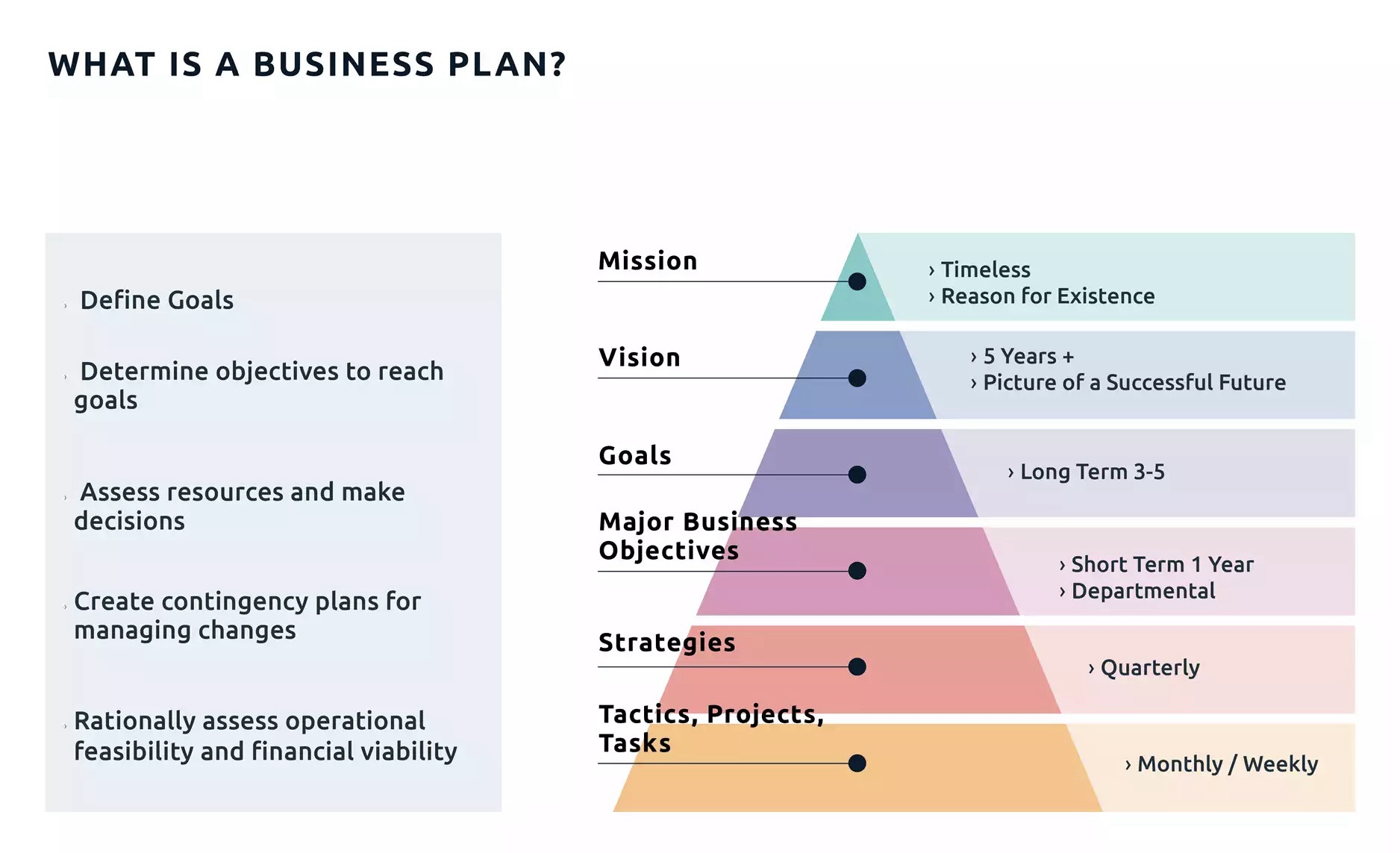
A roadmap is a strategic plan that defines a goal or desired outcome and includes the major steps or milestones needed to reach it. It also serves as a communication tool, a high-level document that helps articulate strategic thinking—the why—behind both the goal and the plan for getting there.

A business roadmap is a visual representation of your business strategy. It outlines the steps, goals, initiatives, and milestones needed to achieve your long-term plans. A business roadmap is also more tactical, focusing on how you will reach your objectives.

Eight Bukets – Challenge

Six – Create Value – Capture Value

I’m giving you the map, now you must walk the path

https://youtu.be/qllWAheHkms?si=fCkbOSRuRO5kZ0ol

The 80 – 20 Rule

https://www.investopedia.com/terms/1/80-20-rule.asp

Posted in software online review

Chromium

https://en.wikipedia.org/wiki/Chromium_(web_browser)

The One Investment Rule

https://youtu.be/IBD_AdM3WNI?si=xORYvpzXfwyYxO-a

Chromium org

https://www.chromium.org/chromium-projects/

browsing history

https://interestingengineering.com/culture/chatgpt-to-absorb-users-life-history

ghat gpt – gemini – missing personality

https://www.tomsguide.com/ai/i-switched-from-chatgpt-to-gemini-for-one-week-and-heres-why-im-going-back-to-chatgpt

Chromium base

https://www.pcmag.com/comparisons/chatgpt-vs-gemini-which-ai-chatbot-is-actually-smarter

Gemini

https://gemini.google.com/app/download

https://gemini.google/subscriptions/

Chat Gpt – Open AI

https://chatgpt.com/

https://openai.com/

https://en.wikipedia.org/wiki/OpenAI